世界での"tofu"に関するトレンド調査
カテゴリー: 大豆蛋白・大豆ミート
投稿日: 2022-08-15
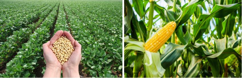
健康、蛋白質供給、環境負荷などから国内では大豆による代替肉、すなわち"大豆ミート"への関心が高まっています。
忘れてならない伝統的大豆タンパク質食品に豆腐があります。
今回は、"tofu"の世界的な関心のトレンドをグーグルトレンドで調べてみました。
調査・解析方法
- 情報源: Googleトレンド
- GoogleトレンドのデータはPythonのPytrendsを使用して取得(コードを記載)
- 検索ワード: "tofu", "tofu near me", "air fryer tofu", "cheese", "meat", "beef"
- Pytrendsのパラメーター:
- 言語設定 英語 hl='en-US'
- タイムゾーン 米国標準時間 tz=360
- 検索地域 すべての国 geo=''
- 検索期間 timeframe='2012-01-01 2022-07-31'
- カテゴリー フード、ドリンク cat=71
Googleトレンド
Goolgeトレンドとは、Googleにおける検索頻度の相対的動向をチェックできるGoogleが提供するツールです。
検索行動から関心の高さのトレンドが推定できます。食品としての関心トレンドに絞り込むために検索カテゴリーを"Food & Drink”に設定しています。
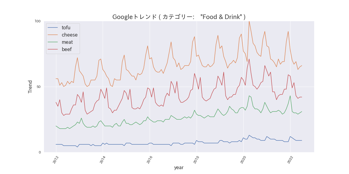
"tofu"のGoogleトレンドを"cheese", "meat", "beef"と比較
cheese,meat,beefなどの動物性タンパク質食品と比べて、tofuも意外に健闘している印象です。直近12ヶ月での比は、tofu:8、cheese:63、meat:37、beef:42です。
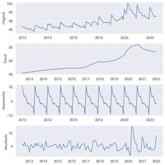
"tofu"のGoogleトレンドをトレンド変動、季節変動、残渣変動の各成分に分ける
Pythonで作成したプログラムで、Googleトレンドのような時系列データの変動は簡単に、トレンド変動、季節変動、残渣変動に分けることができます。
トレンド変動を見ると、"tofu"への関心は2020年まで持続的に増加傾向でしたが、2020年にピークアウトしています。米国発のbeyond meatやimpossible meatなどの植物性の代替肉の出現のためかもしれません。季節変動としては年末に一旦減少して、1月に入って大きく急上昇しています。
"tofu"トレンドの国別ランキング(右側の数字は相対的な検索頻度)
アジア2カ国、北米2カ国、オセアニア2カ国、ヨーロッパ4カ国と英語のtofuの検索頻度では欧米、オセアニアが目立ちます。
- シンガポール 100
- カナダ 83
- ニュージーランド 56
- オーストラリア 56
- フィリピン 51
- アメリカ合衆国 43
- スロバキア 37
- スイス 37
- フィンランド 36
- チェコ 34
"tofu"に関係する検索ワードの頻度ランキング(右側の数値は相対的検索頻度)
検索頻度が高いのは圧倒的にtofuの料理レシピです。
- tofu recipe 100
- tofu recipes 100
- fried tofu 29
- tofu soup 27
- tofu stir fry 25
"tofu"に関係する検索ワードの急上昇頻度ランキング(右側の数値は上昇比です)
- tofu near me 50000
- air fryer tofu 40400
- tofu keto 11550
- is tofu keto 9050
- air fry tofu 8950
急上昇ランキング1位は"tofu near me"で、2位は"air fryer tofu"でした。
実際にChromeの検索設定の言語を英語に、地域を米国に設定してGoogle検索してみると、"tofu near me" では豆腐料理を食べられる店舗サイトが、"air fryer tofu"ではレシピサイトがヒットしました。
豆腐料理への関心が海外でも高いことが伺えます。
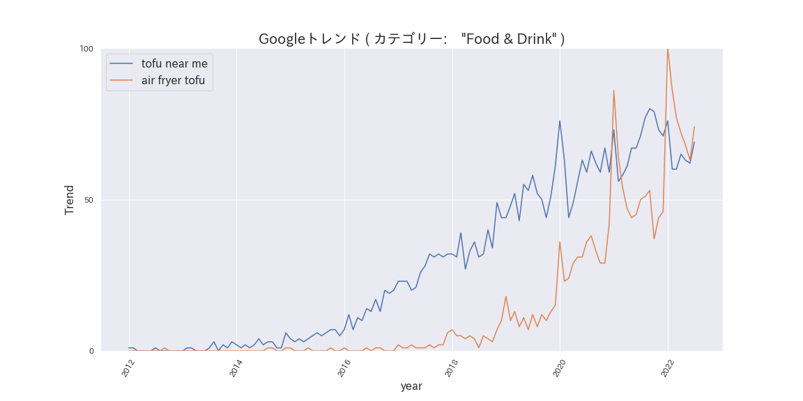
"tofu near me"、"air fryer tofu" のGoogleトレンド
"tofu near me"は2015年頃から、"air fryer tofu"は2018年頃から継続的に上昇傾向です。
Pythonによるプログラムのコード
上記Googleトレンドのプロット作成に用いたPythonのコードです。
Googleトレンドのデータ取得には、ウエブページ上で検索してcsvファイルにダウンロードする方法と、Pythonのライブラリである
Pytrendsを使う方法があります。今回はPytrendsを使うコードを掲載しました。PytrendsはGoogleトレンドの非公式なAPIですので、一度に多量な検索は慎みましょう。
あくまで参考です。自己責任で適当に編集して試してください。
開発・実行環境:Google Colaboratory
InstallとImport
# Install
!pip install pytrends
!pip install japanize-matplotlib

# Import
from pytrends.request import TrendReq
import requests
from lxml import etree
from datetime import datetime, timedelta
import pandas as pd
import numpy as np
import matplotlib.pyplot as plt
import japanize_matplotlib
import seaborn as sns
sns.set(font="IPAexGothic")
import statsmodels.api as sm
検索ワード"tofu", "cheese", "meat", "beef" のGoogleトレンドデータの取得とプロット
# タイムゾーンとキーワード設定  hl='en-US':言語設定 tz=360:US標準時間
pytrends = TrendReq(hl='en-US', tz=360)
kw_list_01 = ['tofu', 'cheese', 'meat', 'beef']

# データ作成 cat=71:フード、ドリンク geo='':全ての国 cat=71:カテゴリーをフード、ドリンクに
pytrends.build_payload(kw_list_01, cat=71, timeframe='2012-01-01 2022-07-31', geo='', gprop='')

# データ取得
df = pytrends.interest_over_time()
df.info()	#取得したデータフレームの確認

## Plot
Y1 = kw_list_01[0]
Y2 = kw_list_01[1]
Y3 = kw_list_01[2]
Y4 = kw_list_01[3]
fig, ax = plt.subplots(figsize=(16, 8))
plt.xticks(rotation=60)
ax.plot(df.index, df[Y1], label = Y1)
ax.plot(df.index, df[Y2], label = Y2)
ax.plot(df.index, df[Y3], label = Y3)
ax.plot(df.index, df[Y4], label = Y4)
ax.set_title('Googleトレンド ( カテゴリー: "Food & Drink" )', fontsize=20)
ax.set_xlabel('year', fontsize=16)
ax.set_ylabel('Trend', fontsize=16)
ax.set_ylim(0, 100)
ax.set_yticks([ 0, 50, 100 ])
ax.set_yticklabels([0, 50, 100 ])
plt.legend(fontsize=16)
plt.show()
"tofu"のGoogleトレンドをトレンド変動、季節変動、残渣変動の各成分に分ける
# Pandas.Seriesにデータを格納(データに乗客数、インデックスは日付)
tofu = pd.Series(df['tofu'], dtype='float')
tofu.index = pd.to_datetime(df.index)

res = sm.tsa.seasonal_decompose(tofu)
original = tofu # オリジナルデータ
trend = res.trend # トレンドデータ
seasonal = res.seasonal # 季節性データ
residual = res.resid # 残差データ

#plot
## グラフ描画枠作成、サイズ指定
plt.figure(figsize=(8, 8))
## オリジナルデータのプロット
plt.subplot(411) # グラフ4行1列の1番目の位置(一番上)
plt.plot(original)
plt.ylabel('Original')
## trend データのプロット
plt.subplot(412) # グラフ4行1列の2番目の位置
plt.plot(trend)
plt.ylabel('Trend')
## seasonalデータ のプロット
plt.subplot(413) # グラフ4行1列の3番目の位置
plt.plot(seasonal)
plt.ylabel('Seasonality')
## residual データのプロット
plt.subplot(414) # グラフ4行1列の4番目の位置(一番下)
plt.plot(residual)
plt.ylabel('Residuals')
## グラフの間隔を自動調整
plt.tight_layout()
"tofu"に関係する検索ワードの頻度ランキングと急上昇ランキング
df_que = pytrends.related_queries()
print(df_que['tofu']['top'].head(10))
print()
print(df_que['tofu']['rising'].head(10))
"tofu near me", "air fryer tofu"のGoogleトレンド
# タイムゾーンとキーワード設定
pytrends = TrendReq(hl='en-US', tz=360)
kw_list_02 = ['tofu near me', 'air fryer tofu']

# データ作成
pytrends.build_payload(kw_list_02, cat=71, timeframe='2012-01-01 2022-07-31', geo='', gprop='')

# Plot
Y1 = kw_list_02[0]
Y2 = kw_list_02[1]
fig, ax = plt.subplots(figsize=(16, 8))
plt.xticks(rotation=60)
ax.plot(df.index, df[Y1], label = Y1)
ax.plot(df.index, df[Y2], label = Y2)
ax.set_title('Googleトレンド ( カテゴリー: "Food & Drink" )', fontsize=20)
ax.set_xlabel('year', fontsize=16)
ax.set_ylabel('Trend', fontsize=16)
ax.set_ylim(0, 100)
ax.set_yticks([ 0, 50, 100 ])
ax.set_yticklabels([0, 50, 100 ])
plt.legend(fontsize=16)
plt.show()
fig.savefig("output/trend_tofu_near_me_air_dryer_tofu.png")